
Note——GRAPH NEURAL NETWORKS WITH LEARNABLE STRUCTURAL AND POSITIONAL REPRESENTATIONS
Published:
Paper Address: Graph Neural Networks with Learnable Structural and Positional Representations
1 What has this paper done?
The authors introduce a new type of learnable positional encoding (PE) of nodes for graph embedding like transformer in natural language processing.
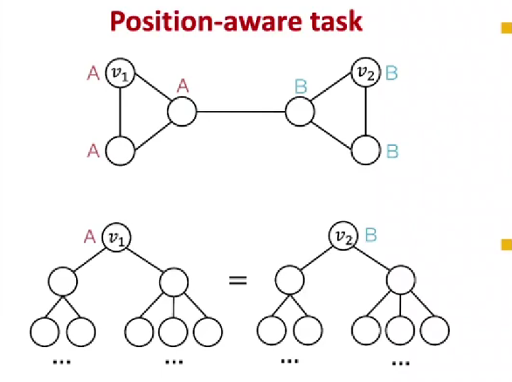
2 Why positional encoding in graph embedding?
Past message-passing mechanism can not distinguish two atoms which are with the same 1-hop neighbors but play separate roles in a graph (like a molecule).
2.1 Previous Solution
stacking multiple layers
It could be deficient for long-distance nodes because of the over-squashing phenomenon.
applying higher-order GNNs
K-orders WL-GNN are computationally more expensive to scale than MP-GNNs, even for medium-sized graphs.
considering positional encoding (PE) of nodes (and edges)
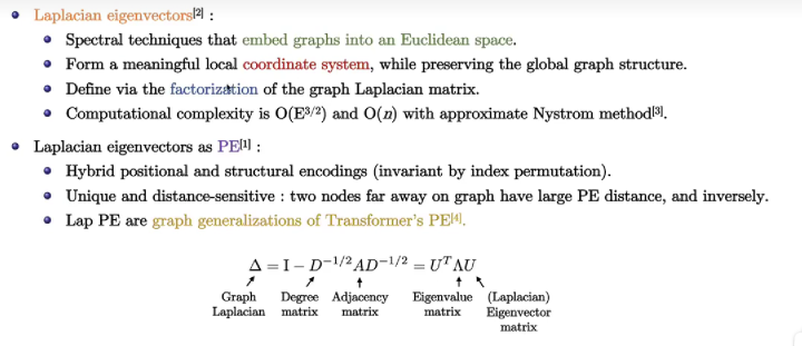
Laplacian Eigenvectors as PE
It is related to the Graph Fourier Transformer, which transforms graph sign into sine. (more information can be found at this blog)
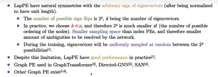
Limitations of Laplacian PE
3 Motivations
decouple structural and positional representations to make easy for the network to learn these two essential properties.
4 Random walk PE
The choice of the initial PE is critical. Due to the sign flips of laplacian PE, the authors proposed random walk positional encoding :
Explaination. The adjacency matrix \(A\) of a graph \(G\), the non-zero elements in \(A\) describe the weight of each edge in the graph \(G\) (here, the diagonal of \(A\) is generally required to be zero). This weight describes the similarity between nodes, however, it is not obvious when the value is 1, so we need to normalize this matrix by row. The resulting matrix \(RW\) is a random walk matrix, which indicates the landing probability of a node \(i\) to other nodes. \(A\) random walk matrix corresponds to a Markov chain, which means that any two states can reach each other.
Advantages. (1) RWPE provide a unique node representation under the condition that each node has a unique \(k\)-hop topological neighborhood for a sufficient large \(k\). (2) RWPE does not suffer from the sign ambiguity of LapPE, so the network is not required to learn additional invariance.
def init_positional_encoding(g, pos_enc_dim, type_init):
    """
        Initializing positional encoding with RWPE
    """

    n = g.number_of_nodes()

    if type_init == 'rand_walk':
        # Geometric diffusion features with Random Walk
        A = g.adjacency_matrix(scipy_fmt="csr") # Get the adjacency matrix
        Dinv = sp.diags(dgl.backend.asnumpy(g.in_degrees()).clip(1) ** -1.0, dtype=float) # D^-1 just undirected graph can be like this

        RW = A * Dinv  # A*D^-1
        M = RW

        # Iterate
        nb_pos_enc = pos_enc_dim
        PE = [torch.from_numpy(M.diagonal()).float()]
        M_power = M
        for _ in range(nb_pos_enc-1):
            # E.g. The first row of M_power means probabilities from node 0 to its neigbors *
            #      The first col of M means probabilities of node 0's neighbors to node 0 =
            #      The landing probability of a node i to itself
            M_power = M_power * M
            PE.append(torch.from_numpy(M_power.diagonal()).float())
        PE = torch.stack(PE,dim=-1)
        # num_node * pos_enc_dim 第一行表示这张图的第一个节点游走了1,2, ... k次之后返回自身的概率
        # 以此作为该节点的位置编码
        g.ndata['pos_enc'] = PE

    return g
5 MP-GNNS-LSPE
5.1 Notions
\[G \text { : a graph with } \mathcal{V} \text { being the set of nodes and } \mathcal{E} \text { the set of edges. }\] \[A \in \mathbb{R}^{n \times n}\text{: Ajacency matrix}\]5.2 Gated GCN-LSPE
Actually, the authors have implemented various GNNs and GCNs with RWPE, here, I will introduce one called GatedGCN-LSPE. (Gate: it is similar with the gate mechanism in LSTM)s
\(\begin{aligned} h^{\ell+1}, e^{\ell+1}, p^{\ell+1} &=\operatorname{GatedGCN}-\operatorname{LSPE}\left(h^{\ell}, e^{\ell}, p^{\ell}\right), h \in \mathbb{R}^{n \times d}, e \in \mathbb{R}^{E \times d}, p \in \mathbb{R}^{n \times d}, \\ \text { with } h_i^{\ell+1} &=h_i^{\ell}+\operatorname{ReLU}\left(\operatorname{BN}\left(A_1^{\ell}\left[\begin{array}{c} h_i^{\ell} \\ p_i^{\ell} \end{array}\right]+\sum_{j \in \mathcal{N}(i)} \eta_{i j}^{\ell} \odot A_2^{\ell}\left[\begin{array}{c} h_j^{\ell} \\ p_j^{\ell} \end{array}\right]\right)\right) \\ e_{i j}^{\ell+1} &=e_{i j}^{\ell}+\operatorname{ReLU}\left(\operatorname{BN}\left(\hat{\eta}_{i j}^{\ell}\right)\right) \\ p_i^{\ell+1} &=p_i^{\ell}+\tanh \left(C_1^{\ell} p_i^{\ell}+\sum_{j \in \mathcal{N}(i)} \eta_{i j}^{\ell} \odot C_2^{\ell} p_j^{\ell}\right) \end{aligned}\)
Here, I will explain all these formulars with the corresponding code
class GatedGCNLSPELayer(nn.Module):
    """
        Param: []
    """
    def __init__(self, input_dim, output_dim, dropout, batch_norm, use_lapeig_loss=False, residual=False):
        super().__init__()
        self.in_channels = input_dim
        self.out_channels = output_dim
        self.dropout = dropout
        self.batch_norm = batch_norm
        self.residual = residual
        self.use_lapeig_loss = use_lapeig_loss

        if input_dim != output_dim:
            self.residual = False

        self.A1 = nn.Linear(input_dim*2, output_dim, bias=True)
        self.A2 = nn.Linear(input_dim*2, output_dim, bias=True)
        self.B1 = nn.Linear(input_dim, output_dim, bias=True)
        self.B2 = nn.Linear(input_dim, output_dim, bias=True)
        self.B3 = nn.Linear(input_dim, output_dim, bias=True)
        self.C1 = nn.Linear(input_dim, output_dim, bias=True)
        self.C2 = nn.Linear(input_dim, output_dim, bias=True)

        self.bn_node_h = nn.BatchNorm1d(output_dim)
        self.bn_node_e = nn.BatchNorm1d(output_dim)
        # self.bn_node_p = nn.BatchNorm1d(output_dim)
Forward():
def forward(self, g, h, p, e, snorm_n):

  with g.local_scope():

      # for residual connection
      h_in = h
      p_in = p
      e_in = e

      # For the h's
      g.ndata['h']  = h
      g.ndata['A1_h'] = self.A1(torch.cat((h, p), -1))
      # self.A2 being used in message_func_for_vij() function
      g.ndata['B1_h'] = self.B1(h)
      g.ndata['B2_h'] = self.B2(h)

      # For the p's
      g.ndata['p'] = p
      g.ndata['C1_p'] = self.C1(p)
      # self.C2 being used in message_func_for_pj() function

      # For the e's
      g.edata['e']  = e
      g.edata['B3_e'] = self.B3(e)

      #--------------------------------------------------------------------------------------#
      # Calculation of h
      g.applB1(h)
      g.ndata['B2_h'] = self.B2(h)

      # For the p's
      g.ndata['p'] = p
      g.ndata['C1_p'] = self.C1(p)
      # self.C2 being used in message_func_for_pj() function

      # For the e's
      g.edata['e']  = e
      g.edata['B3_e'] = self.B3(e)
g.apply_edges(fn.u_add_v('B1_h', 'B2_h', 'B1_B2_h'))
g.edata['hat_eta'] = g.edata['B1_B2_h'] + g.edata['B3_e'] #用当前边的两个节点和该边的信息更新边
g.edata['sigma_hat_eta'] = torch.sigmoid(g.edata['hat_eta'])
g.update_all(fn.copy_e('sigma_hat_eta', 'm'), fn.sum('m', 'sum_sigma_hat_eta')) # sum_j' sigma_hat_eta_ij'
g.apply_edges(self.compute_normalized_eta) # sigma_hat_eta_ij/ sum_j' sigma_hat_eta_ij'
g.apply_edges(self.message_func_for_vij) # v_ij
g.edata['eta_mul_v'] = g.edata['eta_ij'] * g.edata['v_ij'] # eta_ij * v_ij
g.update_all(fn.copy_e('eta_mul_v', 'm'), fn.sum('m', 'sum_eta_v')) # sum_j eta_ij * v_ij
g.ndata['h'] = g.ndata['A1_h'] + g.ndata['sum_eta_v']
g.apply_edges(self.message_func_for_pj) # p_j
g.edata['eta_mul_p'] = g.edata['eta_ij'] * g.edata['C2_pj'] # eta_ij * C2_pj
g.update_all(fn.copy_e('eta_mul_p', 'm'), fn.sum('m', 'sum_eta_p')) # sum_j eta_ij * C2_pj
g.ndata['p'] = g.ndata['C1_p'] + g.ndata['sum_eta_p']
Activation
h = F.relu(h)
e = F.relu(e)
p = torch.tanh(p)
Residual block: avoid over-squashing while stacking multi-layers
if self.residual:
    h = h_in + h
    p = p_in + p
    e = e_in + e
Explaination. For the formal part of \(\operatorname{ Loss}_{\text {LapEig }}(p)\), \(\Delta p\) is the Laplacian Matrix, so \(p^T \Delta p\) can measure the similarity of the two matrix, \(\operatorname{trace}\left(p^T \Delta p\right)\) can transform the similarity matrix into a value. The latter part of this formular is a constraint to ensure orthogonality. So at last, the learnable positional encoding needs to be similar to laplacian matrix ?(I am not sure I am right, if who knows the reasons, welcome to correct it.)
def loss(self, scores, targets):

        # Loss A: Task loss -------------------------------------------------------------
        loss_a = nn.L1Loss()(scores, targets)

        if self.use_lapeig_loss:
            # Loss B: Laplacian Eigenvector Loss --------------------------------------------
            g = self.g
            n = g.number_of_nodes()

            # Laplacian
            A = g.adjacency_matrix(scipy_fmt="csr")
            N = sp.diags(dgl.backend.asnumpy(g.in_degrees()).clip(1) ** -0.5, dtype=float)
            L = sp.eye(n) - N * A * N

            p = g.ndata['p']
            pT = torch.transpose(p, 1, 0)
            loss_b_1 = torch.trace(torch.mm(torch.mm(pT, torch.Tensor(L.todense()).to(self.device)), p))

            # Correct batch-graph wise loss_b_2 implementation; using a block diagonal matrix
            bg = dgl.unbatch(g)
            batch_size = len(bg)
            P = sp.block_diag([bg[i].ndata['p'].detach().cpu() for i in range(batch_size)])
            PTP_In = P.T * P - sp.eye(P.shape[1])
            loss_b_2 = torch.tensor(norm(PTP_In, 'fro')**2).float().to(self.device)

            loss_b = ( loss_b_1 + self.lambda_loss * loss_b_2 ) / ( self.pos_enc_dim * batch_size * n)

            del bg, P, PTP_In, loss_b_1, loss_b_2

            loss = loss_a + self.alpha_loss * loss_b
        else:
            loss = loss_a

        return loss
6 Experiment
6.1 Dataset
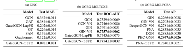
ZINC, OGBG-MOLTOX21, OGBG-MOLPCBA: These datasets, each having a global graph-level property to be predicted, consist of molecules which are represented as graphs of atoms as nodes and bonds between the atoms as edges.
MDB-MULTI, IMDB-BINARY and CIFAR10 superpixels: 3 non-molecular graph dataset, and the datasets used are from the domains of social network.
6.2 Result
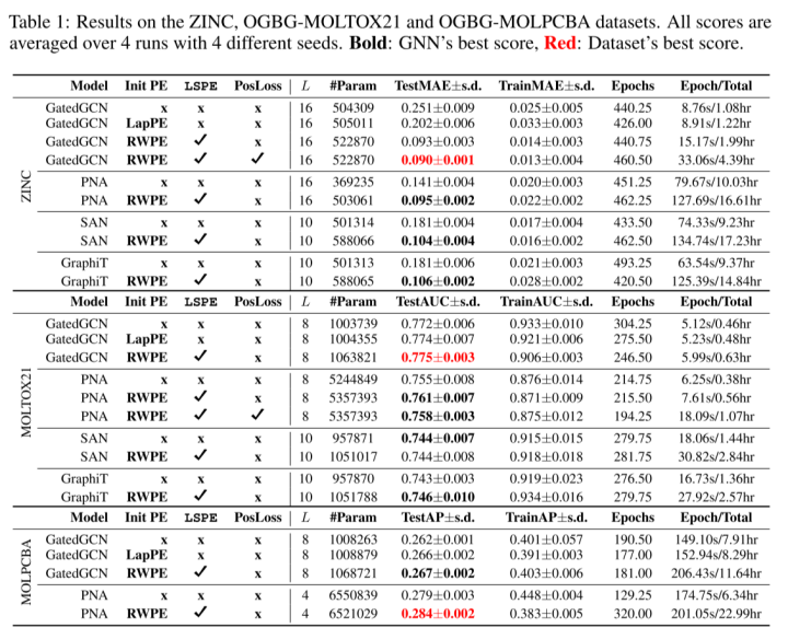
The authors also compare sparse GNN and Transformer GNNs. Sparse GNN achieves better results with LSPE, although Transformer GNN can theoretically better overcome the limitations of long-range dependencies.
References
[1] 阿泽:【GNN】万字长文带你入门 GCN
[2] 马东什么:关于GNN上的position信息利用的一些工作(待续)
[3] Bresson教授图神经网络系列讲座4 GNNs with Learnable Structural and Positional Reps._哔哩哔哩_bilibili
[4] Github: https://github.com/vijaydwivedi75/gnn-lspe
[5] Residual Gated Graph ConvNets
[6] Benchmarking Graph Neural Networks
[7] Cyril-KI:深入理解拉普拉斯特征映射